When I first started reading about machine learning (ML) I thought that ML has two branches – supervised ML (classification) and unsupervised ML (clustering). Today I know better than that and as I have heard a couple of extremely smart and knowledgeable people say, there are roughly 5 types of ML: classification, clustering, decision trees, density estimation and principal component analysis (PCA). Something that I have learnt and intrigued me immensely is that decision trees can be used both in the case of clustering and classification.. Wow, how awesome is that? My answer – pretty darn awesome.
In this blog, I will discuss decision trees only in the context of classification, or supervised machine learning. As the lecture that taught me everything started, I will give you a decision tree as an example so that we have a good understanding of what we are dealing with:
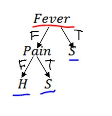
Figure 1.: Example Decision Tree
Each decision tree consists of nodes and edges. When taking a decision, we travel down the nodes of the decision tree following the edges, whose labels correspond to the reality of our current example. Let´s take a step back. On Figure 1., we have 5 nodes of the decision tree – Fever, Pain, S, H, S. The underlined with red node is called the root, and the nodes that have no edges (arrows) going out of them are calledleaves. A decision tree can have only one root. Naturally, a decision tree can have many leaves as in the current example we have S, H and S (standing for sick, healthy and sick). The decision tree has 4 edges represented by the arrows in Figure 1. with respective labels attached to them. All possible labels of the edges of the tree are F, T, F and T, which stand for false, true, false and true.
As you can see the decision tree on Figure 1. can give us a way of diagnosing whether a person is sick or not based on the presence of a couple of factors – checking whether the person has fever or pain can help us decide on this person´s health. Even though this is a very simple example, I hope it helps you get an idea of what we are dealing with here. To generalize things up, following a sequence of decisions from the root of the decision tree we can arrive at a leaf node, which is labelled with the output class of the tree for a particular input pattern. In this case the decision tree is a classification algorithm, and for the example shown in Figure 1., the decision tree helps us differentiate between two classes – S (sick) and H (healthy).
Decision trees describe a decision method. Some of you might be well familiar with machine learning already, and therefore it is important to note that the nomenclature in the case of decision trees differs from other learning algorithms. This is because decision trees were used even before machine learning formed as an area of research and interest. Each node of a decision tree tests an attribute of this decision tree. Depending on the number of attributes we test in the decision tree, we can say that the input patterns for our learning are formed by a number of components, this number being the number of attributes. For the decision tree in Figure 1., the input pattern is formed by two components (or two attributes – binary in this case). We can also have numerical attributes, different than true and false. We already spoke about the root of the tree and the leaves of the tree, but it is also important to note that all other nodes are called attribute nodes. In Figure 1. we can see only one attribute node, that is the one that tests the attribute Pain.
One remark that I heard in the middle of the lecture and I think it is important nevertheless not related to decision trees is the following. In the general case SVMs work better than MLPs (Multi-layer Perceptrons, the other name for Neural Networks) for data of reasonable sizes. As it turns out MLPs perform better when assessing credit risk, but due to their mathematical complexity, the reasoning behind their prediction is difficult to be explained to the general public. In addition, if we have very very large sets of data, the optimization of the MLPs becomes tricky and slow so their use is not advisable. Following this line of logic, decision trees are useful in the cases when it must be easy to explain to someone how it is working and why is the learning algorithm predicting what it predicts. Decision forests can also be applied in such cases, and also when we have a large amount of data, which allow us to train multiple classifiers with subsets of the data and use majority voting to predict the final output.
Decision Tree Learning:
A heuristics to train decision trees has been proposed by Ross Quinlan, who developed the ID3 method. Following to that research, Quinlan developed an extension to the ID3 method later in his career that is called C4.5.
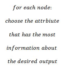
Until the rest of the blog post I will be speaking about ID3 for discrete attributes. The basic idea behind ID3 is that it builds a node at a time starting with the root. It is a conceptually very simple algorithm. It can be summarized in one sentence as follows:
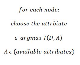
This means we are looking for the Mutual Information between the attribute and the desired output. We can rephrase this into:
where D is the desired output seen as a random variable, and I(D, A) is the Mutual Information between D and A.
I will stop writing for today as I will need to speak about Entropy and Mutual Information to be able to continue describing the decision tree learning. What is left of this blog post is to finish discussing the construction of a decision tree and to see how we prune decision trees. Please send me an e-mail if I take too long to finish it: estambolieva@gmail.com.
Final Notes: This blog post would not be possible without listening to the lecture of Prof. L. B. Almeida from IST in Lisbon. I highly recommend his lectures to anyone who is around and is eager to learn and listen to a good lecturer.


